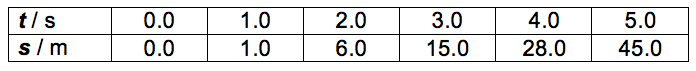
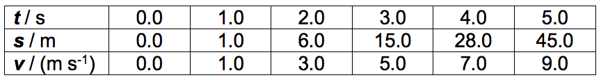
3.5.1 – Tabulated Data Questions | Physics with Mr Shone

A table of data is frequently provided such as the following.

This information could also have been presented to us graphically like so:

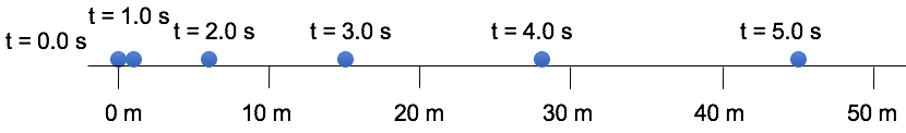
We shall assume that the object is moving in a straight line.

Although the table seems to be only giving information on the distance and time of the object we can in fact use the information to find out other aspects of the motion.

Looking at the first second (between t=0.0 s and t=1.0 s) we can see that the object moves a distance of 1.0 m giving an average velocity of 1.0 m/s over the first second.

Similary, for the second second (between t=1.0 s and t=2.0 s) we can see that the object moves a distance of 5.0 m (moving from 1.0 m to 6.0 m positions) giving an average velocity of 5.0 m/s over the second second.

We can do this for all the time intervals and end up with a new row of data as shown here:

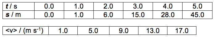
Notice that in the new row the columns do not line up with the above table. They aren’t supposed to. The average velocity of 9.0 m/s does not occur at t =2.0 s or a time t=3.0 s, but is an average velocity over the whole one second time interval. (In fact we will often take it to be the instantaneous velocity at the midpoint. i.e. at t=2.5 s)

This new row tells us that the velocity is not constant, but is increasing. i.e there is an acceleration.

From the new row we have created in the table we can see that at t=0.5 s the average velocity is 1.0 m s^-1, and at t=1.5 s the average velocity is 5.0 m s^-1. So the velocity changes by 4.0 m/s in this time interval. The time interval in this case is of course 1.0 second (1.5 s – 0.5 s = 1.0 s)

Thus the average acceleration over this time period is 4.0 m s^-2.

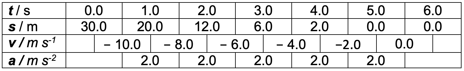
We can apply the same logic to the other changes in velocity and end up with the following:

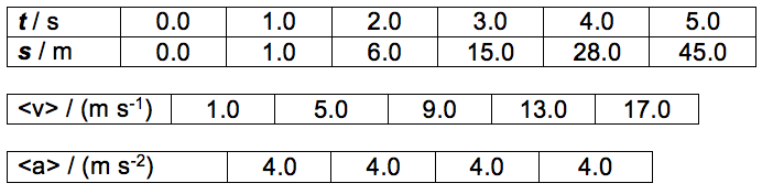
So we can conclude that the acceleration is uniform for this object over these 5.0 seconds.

A Common Mistake
A common mistake is to calculate the table as such: Can you figure out what these values actually represent? 9.0 obviously comes from 45.0 ÷ 5.0 = 9.0 This IS an average velocity, however, it is the average over the whole 5.0 s and so represents the velocity that the object possessed at t=2.5 S.

A Common Mistake

A common mistake is to calculate the table as such:

Can you figure out what these values actually represent?

9.0 obviously comes from 45.0 ÷ 5.0 = 9.0

This IS an average velocity, however, it is the average over the whole 5.0 s and so represents the velocity that the object possessed at t=2.5 S.

Note
Of course the table will not always consist of time and displacement values. Time and velocity data is frequently given, and sometimes even time and acceleration data.

Example
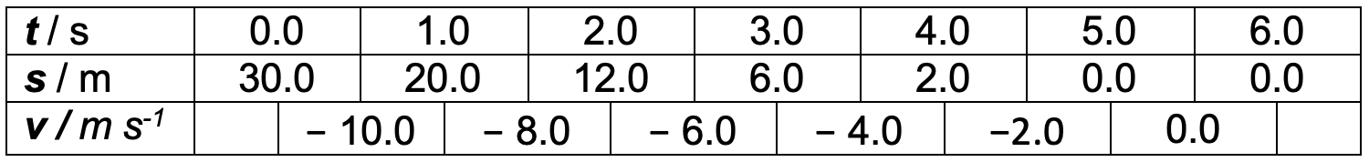
The table below shows data for a car along a straight road from the starting point of the road. The table below shows variation of time t and the displacement s of the car. *(a) State, giving your reasons, whether the speed of the car is increasing, decreasing* or remaining constant, Adding a lower row to the table we can determine the velocity of the car at different intervals: Thus the speed of the car can be seen to be decreasing** (i.e. the car is slowing down) Note the values of v are negative here as the displacement is decreasing (eg. in the first second the displacement goes from 30 m down to 20 m – so the change in displacement is 20-30 = −10 m.) (b) State, giving your reasons, whether the acceleration of the car is increasing, decreasing or remaining constant Adding a further lower row to the table we can determine the acceleration of the car at different intervals: Thus the acceleration of the car can be seen to be constant. Note the values of a are positive here. (eg. as the velocity changes from −10 m s⁻¹ to −8 m s⁻¹ the change in velocity is −8.0–(−10.0)=+2.0 m s⁻¹.)

Example

The table below shows data for a car along a straight road from the starting point of the road. The table below shows variation of time t and the displacement s of the car.

(a) State, giving your reasons, whether the speed of the car is increasing, decreasing or remaining constant,

Adding a lower row to the table we can determine the velocity of the car at different intervals:

Thus the speed of the car can be seen to be decreasing (i.e. the car is slowing down)

Note the values of v are negative here as the displacement is decreasing (eg. in the first second the displacement goes from 30 m down to 20 m – so the change in displacement is 20-30 = −10 m.)

(b) State, giving your reasons, whether the acceleration of the car is increasing, decreasing or remaining constant

Adding a further lower row to the table we can determine the acceleration of the car at different intervals:

Thus the acceleration of the car can be seen to be constant.

Note the values of a are positive here. (eg. as the velocity changes from −10 m s⁻¹ to −8 m s⁻¹ the change in velocity is −8.0–(−10.0)=+2.0 m s⁻¹.)

2025 Physics Lessons