- In this section, although we will frequently be referencing an oscilloscope, a data-logger will display similar results and will have similar controls.
- You may also see references to a cathode ray oscilloscope (c.r.o. for short), this technology has been replaced and all oscilloscopes you come across now are likely to be digital displays and not based on a cathode-ray tube.
- When a sound travels to a microphone connected to an oscilloscope, the microphone converts the sound energy into electrical signals. The oscilloscope displays the waveform of the signals on a screen.
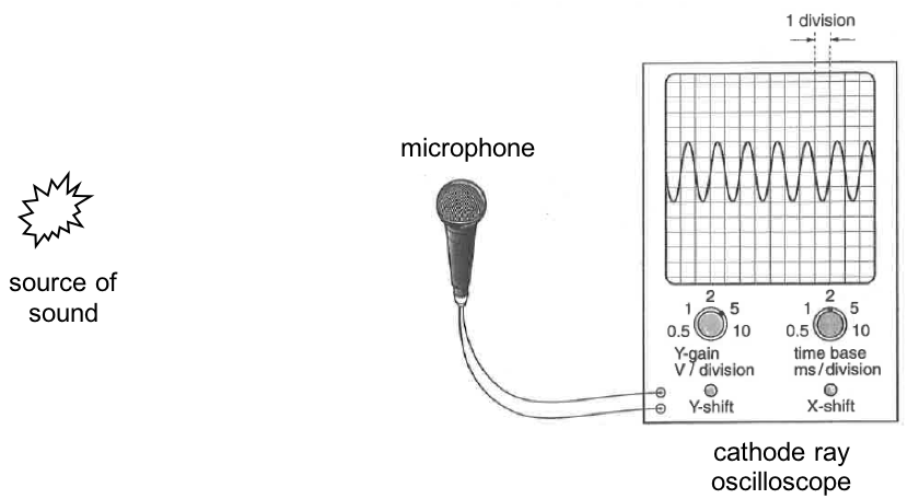
- The oscilloscope has controls to display the characteristics of the waveform (e.g. amplitude, period).
Displaying waveforms
- Oscilloscopes are widely used for displaying waveforms (e.g. sound waveforms from a microphone). By selecting a suitable scale for the gain, we can display the voltage waveform by connecting to the Y-terminal input.
| Note |
|---|
| Don’t worry about the workings of a c.r.o. you won’t be tested on that.
Understand that the screen display can be though of as is essentially just a graph. Amplitude (as measured by input voltage) on the Y-axis and time along the X-axis. |
Measuring Voltages, Short Intervals of Time and Frequencies
1. DC Input, Time-base Off
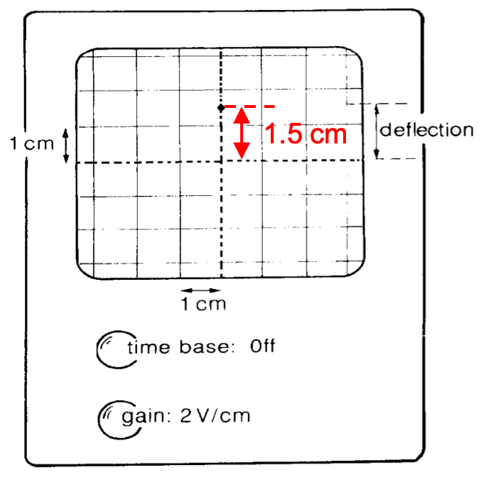 With a constant voltage (direct current – d.c.) input (e.g. a battery) connected to the Y-terminals and the time-base turned off the dot will just move in the vertical direction.
This oscilloscope is showing a voltage of 1.5 cm × 2 V/cm = 3.0 V
2. AC Input, Time-base Off
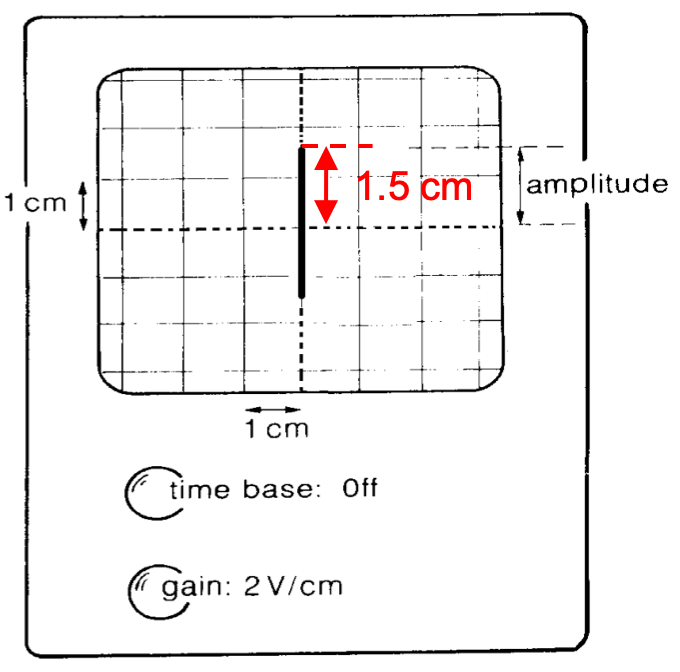 With the input voltage now changed to an alternating current (a.c) the dot will oscillate up and down. If the oscillations are fast enough it will simply appear as a line.
This oscilloscope is showing a peak-peak voltage of 3.0 cm × 2 V/cm = 6.0 V
i.e the wave has an amplitude of 3.0 V.
3. AC Input, Time-base On
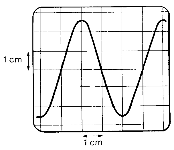
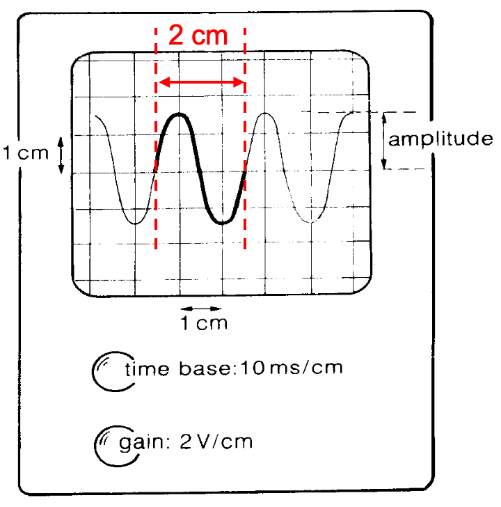 With the timebase now turned on, the dot will also sweep left to right. Here we can see the wave completes one cycle in 2 .0 cm corresponding to a period of 20 ms.
This oscilloscope is showing a peak-peak voltage of 3.0 cm × 2 V/cm = 6.0 V
As the horizontal scale is time, measuring one wave will give us a period, T.
Period = 2.0 cm × 10 ms/cm = 20 ms (0.020 s)
The frequency can be determined in the usual way from ƒ=1/T.
ƒ=1/T ƒ=1/0.020 = 50 Hz
| Example |
|---|
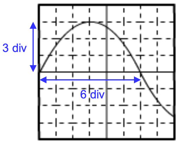
| The diagram below shows the waveform of an a.c. supply displayed on an oscilloscope.
If the gain control is set to 50 mV / cm and the time base control set to 10 ms / cm, determine: the peak-to-peak voltage of the a.c. supply = 5 cm x 50 mV = 250 mV (b) the peak voltage of the a.c. supply. the peak voltage of the a.c. supply = ½ x 250 mV =125 mV (c) the frequency of the a.c. supply. the frequency of the a.c. supply. Period, T = 4 cm x 10 ms = 40 ms Frequency = 1/T = 1/0.040 = 25 Hz
|
| Example |
|---|
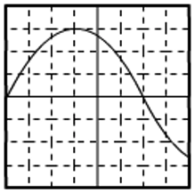
| The screen of an oscilloscope is shown in the figure below.
The Y-plates are connected to an a.c. supply. The following settings are used. Y-gain setting = 2.0 V / division Time-base setting = 1.0 ms / division
(a) Calculate the frequency of the wave
(b) If the time-base is changed to 3.0 ms / division and the Y-gain is changed to 1.5 V / division, draw the new waveform. |
| Waves & Sound |