Microsoft Excel is a great way to check your choice of best-fit line or your gradient calculation.
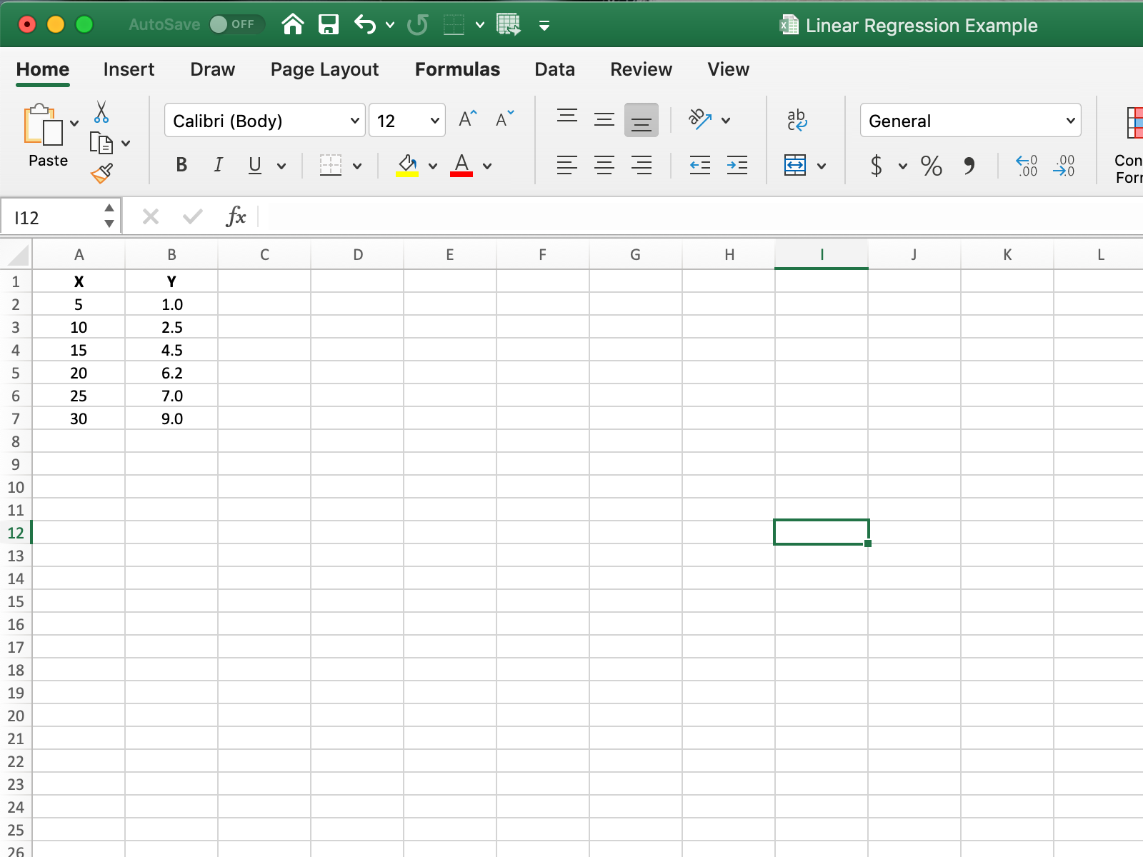
- Type in the data from your table
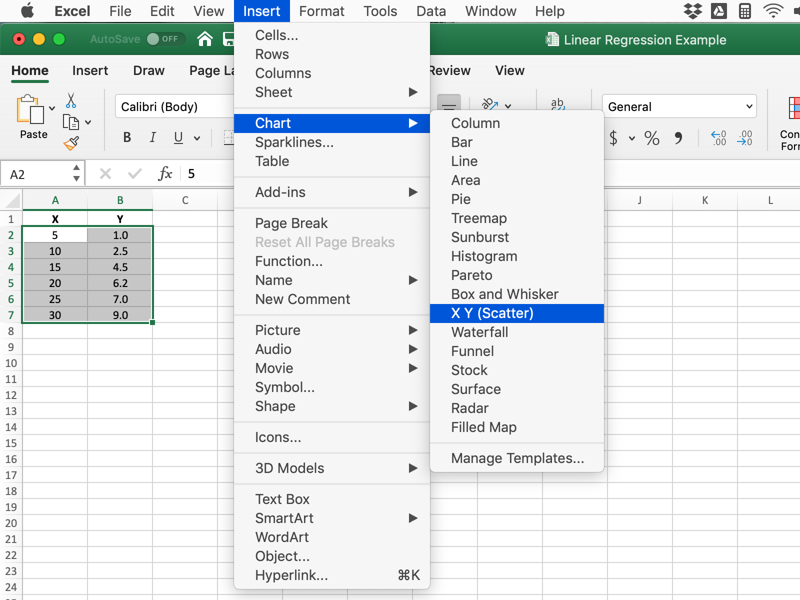
2. Highlight the data to be plotted and then select Insert >> Chart >> X Y (Scatter)
3. Your graph should appear like this.
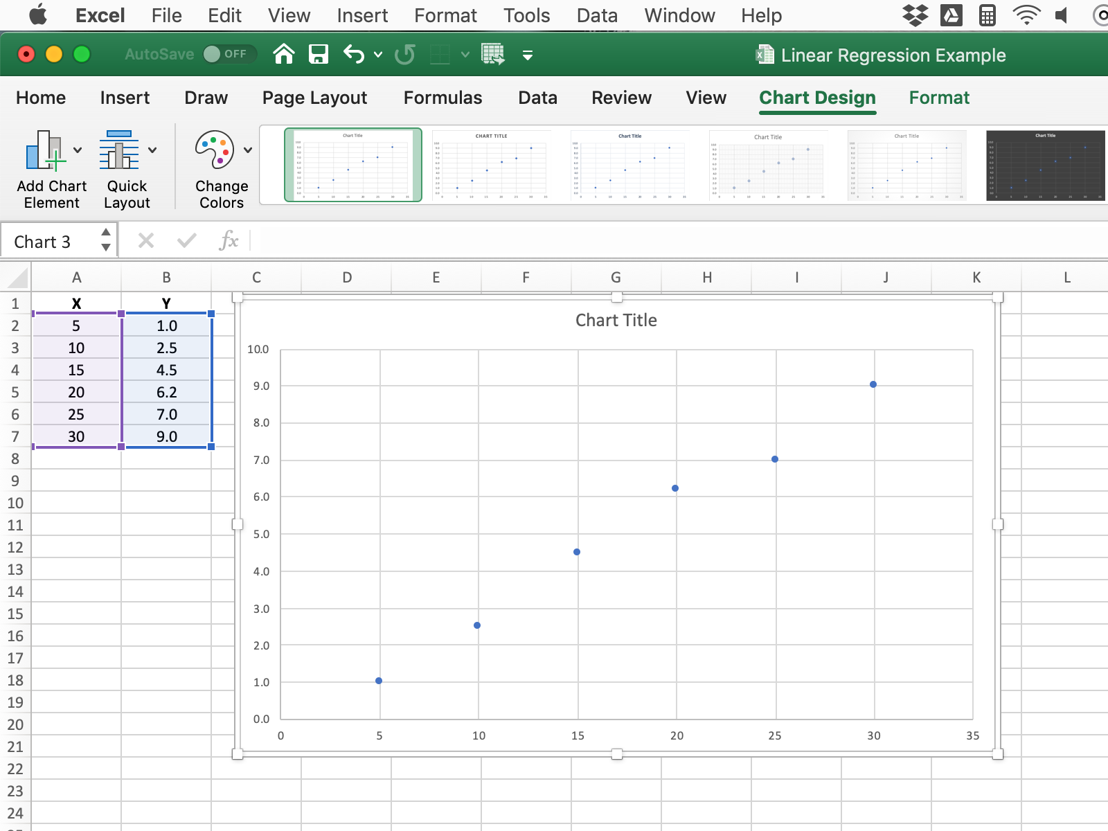
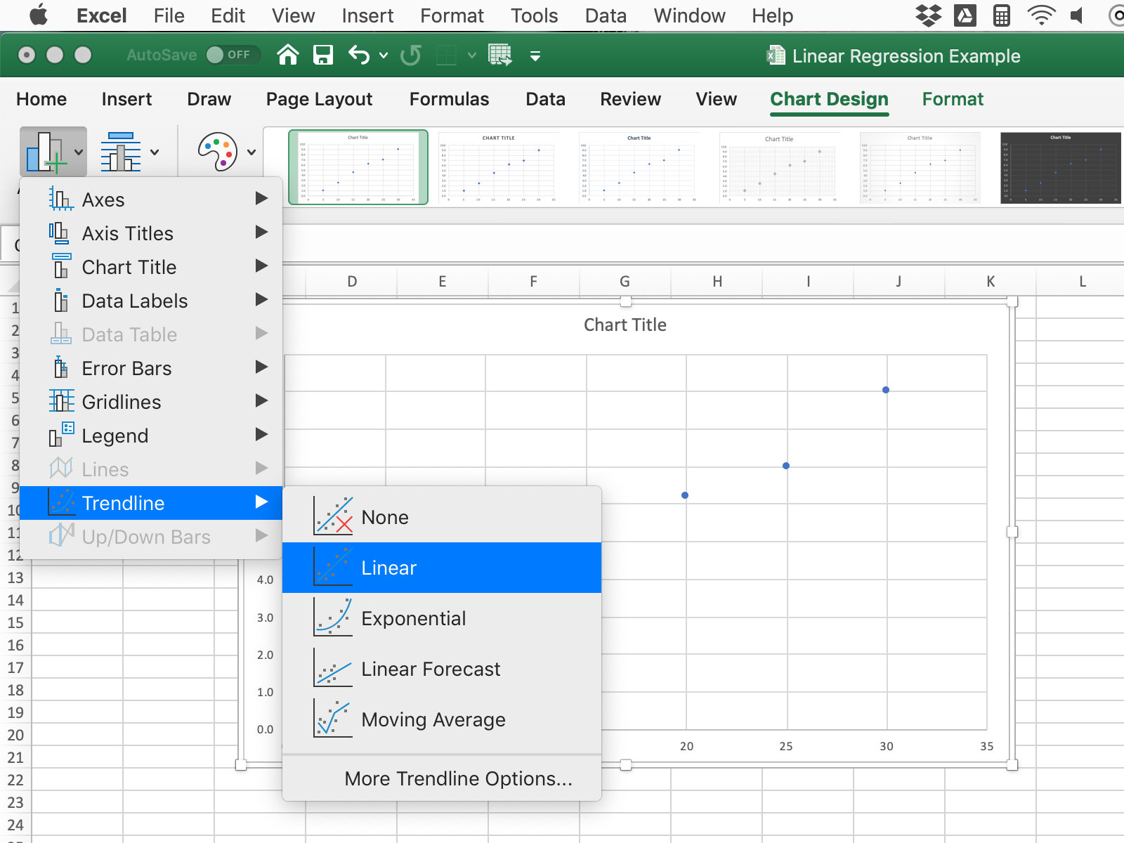
4. To add a best-fit line select Chart Design >> Add Chart Element >> Trendline >> Linear
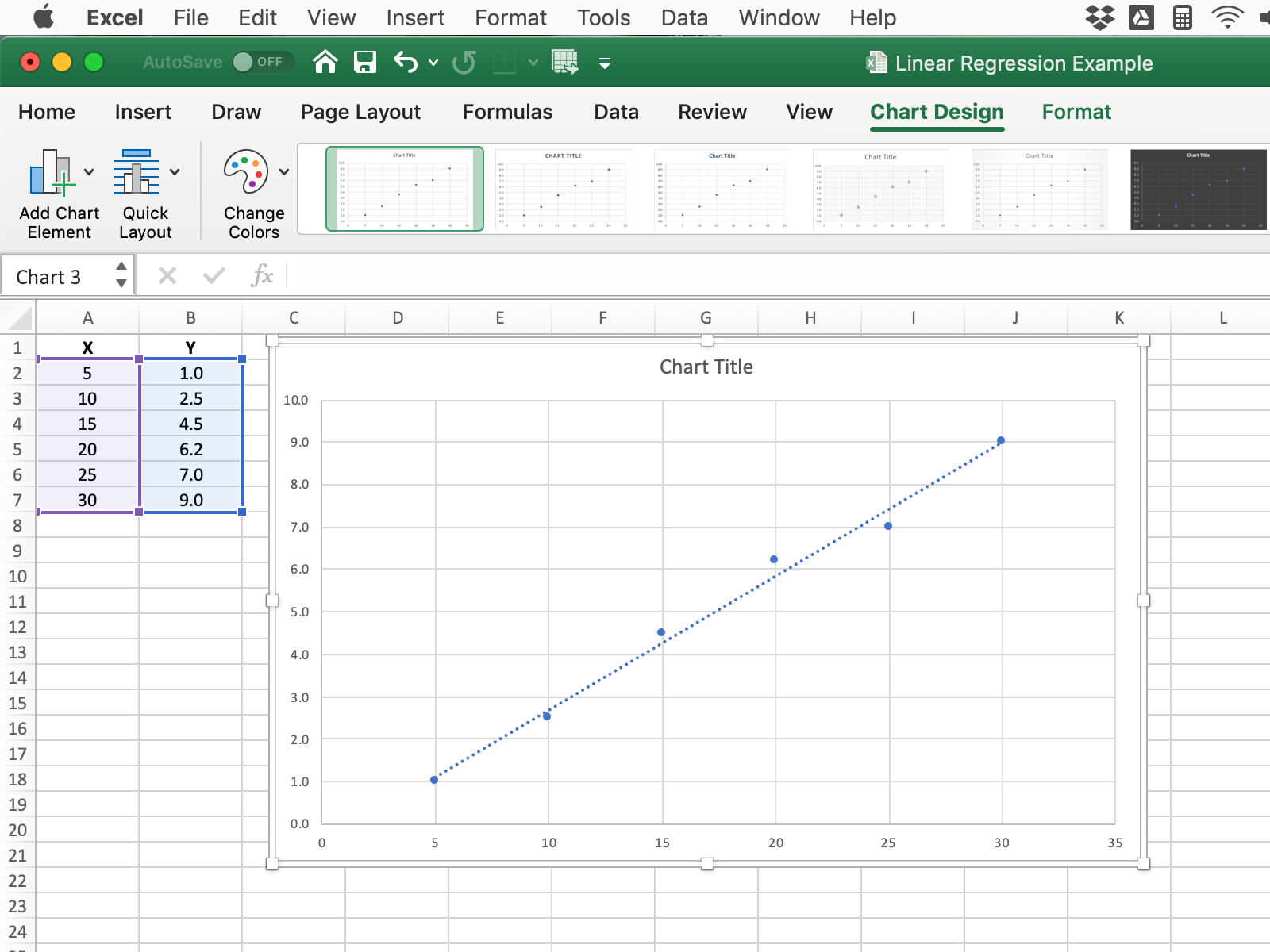
5. Your graph will now look like this.
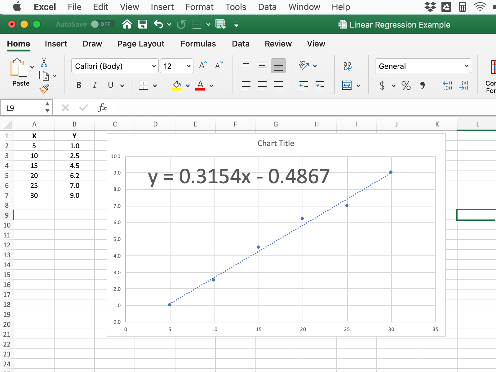
Right click on the best-fit line and select Format Trendline to see the following. Select Display Equation on chart
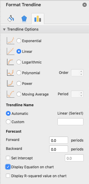
You will now see something like this.
The gradient of this graph is thus 0.3154 (as the equation is in the form y=mx + c)